
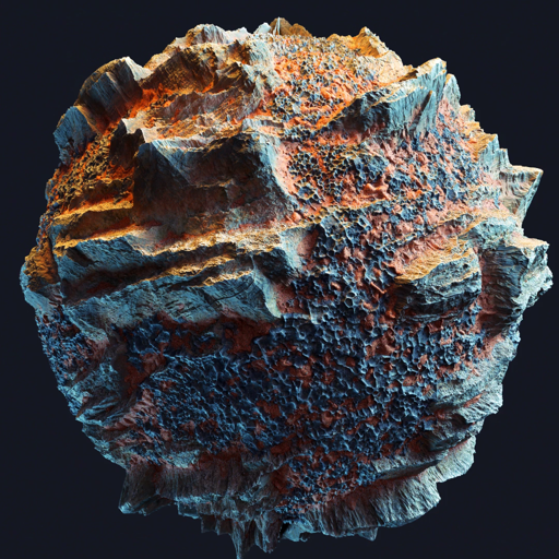
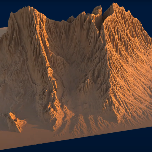
Procedural Island Generation (III)
Sep 17, 2025
Adding multi-scale noise layers, mountain distance fields, and elevation blending to create detailed terrain from the paint map foundation.

Procedural Island Generation (II)
Sep 10, 2025
Creating terrain elevation with a paint map system, mountain ridges, and custom color gradients for natural-looking procedural islands.

Procedural Island Generation (I)
Sep 7, 2025
Building the foundation for procedural island generation with Voronoi diagrams, Delaunay triangulation, and a paint map system for terrain specification.

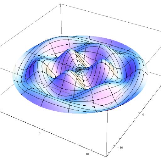
Aug 25, 2025
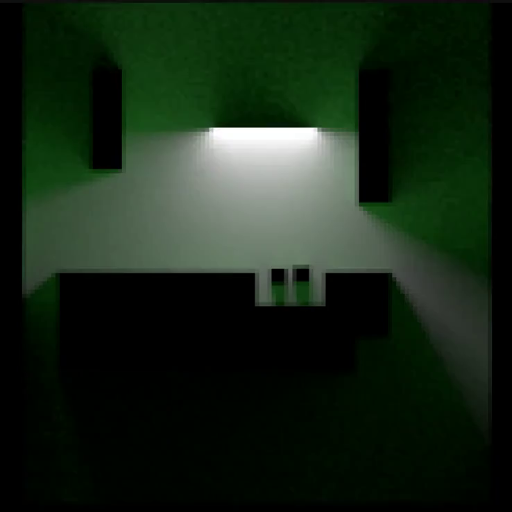
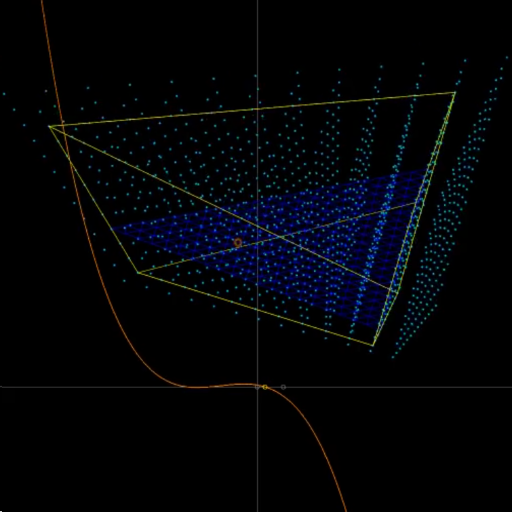
A math tool you can use to encode/decode the radiance arriving at a point with just a few coeffs.
Sep 5, 2023
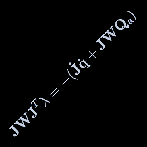
Direct continuation to the force-based constraint posts: Systems of constraints.
Aug 14, 2023
A new entry in my constrained dynamics series. Force-based constraints.

Aug 4, 2023
A new entry in my constrained dynamics series. Springs are a no-go for constraints.

Jul 30, 2023
Introductory entry in my series of posts about constrained dynamics.
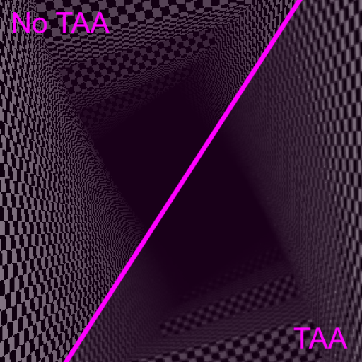
Reprojection Temporal Anti-Aliasing
May 6, 2023
Description and full Shadertoy implementation of a TAA system.
Micro-Patch Displacement Mapping
Sep 30, 2022
An overview of Maverick Render's new Micro-Patch Displacement Mapping system.
Diffraction vs. Multi-resolution
Sep 29, 2022
Comparison of diffraction effects in Maverick Render at multiple resolutions.
Sep 22, 2022
Some technical flybys from Maverick Render's displacement mapping system.

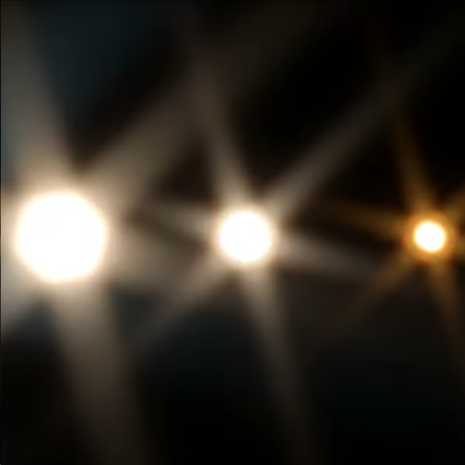
Glare/Bloom versatility in Maverick
Sep 16, 2022
Miscellaneous examples of diffraction effects in Maverick Render.
Fourier Transform of a unit pulse
Sep 5, 2022
Mathematical derivation of the Fourier Transform when the input signal is a unit pulse.
Playing with the Fourier Transform (II)
Sep 4, 2022
What happens to the Fourier Transform when you apply affine transforms to the input signal?
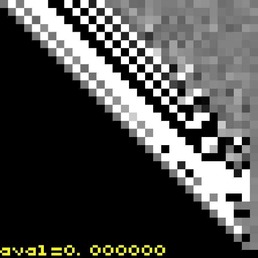
Aug 29, 2022
Full Shadertoy implementation of an avalanche effect tester for 32-bit hash functions.
Octahedron unit-vector encoding
Jul 7, 2022
Different methods of encoding an unit-vector into fewer bits than just 3 floats.
Barycentric coords in triangle sweeps
Jun 18, 2022
An encounter with cubic equations when doing raytracing in swept triangles.
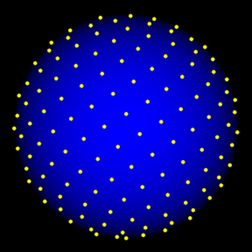
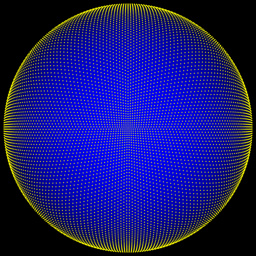
QRNs in the unit square/disk/sphere
May 30, 2022
Transforming pairs of [0..1) numbers between the unit square and the unit sphere.