Fast convolutions (I)
In a previous post it was stated that the convolution of a WxH image with a wxh kernel is a new WxH image where each pixel is the sum of wxh products obtained as the central pixel of the kernel slides across each of the pixels in the original image. This double-double loop leads to an impractical O(n^4) algorithm complexity.
Fortunately, we can do better, but the key here is not in optimizing the code, but in making use of some mathematical weaponry. Let’s analyze the options that we have:
- Naive implementation.
- Separable convolution kernels.
- The convolution theorem.
- Can we do EVEN better?
Naive implementation
Pros:
- Trivial implementation in just a few lines of code.
- Works for any input size, and for any type of kernel.
- Trivial clamping at the boundaries.
- Allows for multi-threading.
Cons:
- Embarrassingly inefficient:
O(n^4). - Requires an auxiliary
WxHbuffer. - By default, the output of the operation is returned in the auxiliary buffer (not in-place).
- Not very cache friendly due to the constant jumps across rows. – Applying the same kernel multiple times has the same cost, every time.
When should I use this method?
- Never, unless the input data is tiny and clean code is more important than sheer performance.
Separable convolution kernels
A separable convolution kernel is one that can be broken into two 1D (vertical and horizontal) projections. For these projections the (matrix) product of the 1xh vertical kernel by the wx1 horizontal kernel must restore the original wxh 2D kernel.
1D vertical and horizontal Gaussian convolution

Conveniently enough, the most usual convolution kernels (e.g., Gaussian blur, box blur, …) happen to be separable.
The convolution of an image by a separable convolution kernel becomes the following:
- Convolute the rows of the original image with the horizontal kernel projection.
- Convolute the columns of the resulting image with the vertical kernel projection.
Note: These two steps are commutative.
2-step separable vs. brute-force 2D Gaussian convolution

Pros:
- More efficient than the naive implementation:
O(n^3). - Trivial implementation in just a few lines of code.
- Trivial clamping at the boundaries.
- Works for any input size.
- Since this is a two-step process, the convolution can be returned in-place.
- Cache-friendly.
- Allows for multi-threading.
Cons:
- Only works with separable kernels.
- Needs an auxiliary
WxHbuffer. - Applying the same kernel multiple times has the same cost, every time.
When should I use this method?
- We do not use this method anywhere in Maverick’s API. You will understand why soon.
The convolution theorem
“The convolution in the spatial domain is equivalent to a point-wise product in the frequency domain, and vice-versa.”
This method relies on the (Fast) Fourier Transform, which is one of the most beautiful mathematical constructs, ever. Seriously!
The convolution of an image by a generic kernel becomes the following:
- Compute the Fourier Transform of the image.
- Compute the Fourier Transform of the kernel.
- Multiply both Fourier Transforms, point-wise.
- Compute the Inverse Fourier Transform of the result.
Brute-force 2D Gaussian vs. the convolution theorem
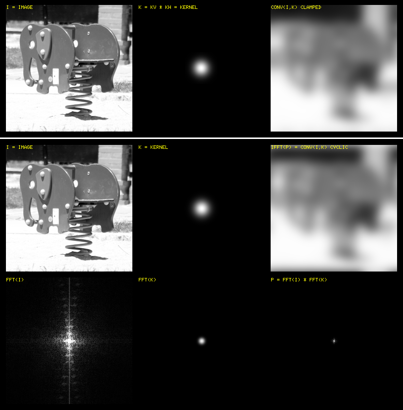
Magic

Pros:
- Even more efficient:
O(n^2·log(n)). - Works with any convolution kernel, separable or not.
- Should the kernel be applied multiple times, the FFT of the kernel can be computed just once, and then be re-used.
- The FFT/IFFT and the convolution product are cache-friendly.
- The FFT/IFFT and the convolution product allow for multi-threading.
Cons:
- Definitely not easy to implement, unless you already own an FFT module that suits your needs.
- The FFT operates on buffers with power-of-2 dimensions. This means that the input image (and the kernel) must be padded with zeroes to a larger size (i.e., extra setup time + memory).
- Both the image and the kernel are transformed, which requires two auxiliary buffers instead of one.
- Each FFT produces complex-number values, which doubles the memory usage of each auxiliary buffer.
- The dynamic range of the FFT values is generally wilder than that of the original image. This requires a careful implementation, and the use of floating-point math regardless of the bit-depth and range of the input image.
- This method doesn’t do any clamping at the boundaries of the image, producing a very annoying warp-around effect that may need special handling (e.g., more padding).
When should I use this method?
- Every time that a large generic convolution kernel (i.e., not a simple blur) is involved.
- The most obvious examples I can think of in Maverick’s are Glare & Bloom.
Can we do EVEN better?
Oh yes. We can do much better, at least in the very particular case of blur. I will talk about this in detail in a dedicated blog entry, at some point.
Some implementation remarks:
All the algorithms presented above allow for multi-threading. Naturally, MT does not change the algorithm complexity, since the maximum number of threads is fixed, but you can get very decent speeds in practical cases if you combine sleek code with proper multi-threading. In the separable case (2), MT must be used twice. First for the rows, and then for the cols. In the FFT case (3), the FFT itself can be multi-threaded (in a rows/cols fashion as well). The huge point-wise product in frequency space can be MT’ed too.
Since convolutions are usually applied on very large images, writing cache-friendly code can make a big difference. Assuming that the memory layout of your image/kernel is per rows, make sure to arrange your loops so memory accesses are as consecutive as possible. This is immediate for the loops that do a 1D convolution on each row. However, for the loops that do a 1D convolution on each column, it may help to use a local cache to transpose a column to a row back and forth.