Point-Spread Functions & Convolutions
One might explain what a convolution is in many ways. However, in the field of image processing, there is an informal and very intuitive way to understand convolutions through the concept of Point-Spread Functions and their inverses.
A PSF is an arbitrary description of the way in which a point spreads its energy around itself in 2D space.
Classic PSFs: 1D box, 2D box, 1D Gaussian, 2D Gaussian
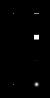
Although this is not a mandatory requirement, the integral of a PSF usually equals 1, so no energy is gained or lost in the process. The above image does not match this requirement for the sake of visualization; the PSFs on the right column have been un-normalized for better visibility. On the other hand, the range of a PSF (how far away from the source point energy is allowed to reach) can be infinite. However, in most practical uses the range is finite, and usually as short as possible.
So, a PSF(x,y) is a function f:R^2->R or, in the case of images, a finite/discrete real-value 2D matrix. For example, PSF(x,y)=0.2 means that the point P=(a,b) sends 20% of its energy to point Q=(a+x,b+y).
If we apply the above PSFs to all the pixels in an image, this is what we get:
Classic PSFs applied to an image

WARNING: Do not confuse this with a convolution; we’re not there yet.
The inverse of a PSF (let’s use the term IPSF for now) is a description of what amount of energy a point receives from the points around itself in 2D space.
So, an IPSF(x,y) is also a function f:R^2->R or, in the case of images, a finite/discrete real-value 2D matrix. For example, IPSF(x,y)=0.2 means that the point Q=(a,b) receives 20% of the energy from point P=(a+x,b+y).
From here follows that a PSF and the corresponding IPSF are radially symmetric:
IPSF(-x,-y) = PSF(x,y)
If P=(a,b) spreads energy to Q=(a+x,b+y), then Q=(a’,b’) gathers energy from P=(a’-x,b’-y).
Finally: a convolution is the result of applying the same IPSF to all the pixels of an image. Note that IPSF matrices are more commonly known as convolution kernels, or filter kernels.
Conveniently enough, the PSFs displayed above are all radially symmetric with respect to themselves. As a matter of fact, it is true to most popular convolution kernels (e.g., 1D/2D box blur, 1D/2D Gaussian blur, …) that the PSF and the IPSF are identical. This makes the process of spreading/gathering energy equivalent in the cases presented above, but this is not true to other (more exotic) kernels.
In the case of image convolutions, kernels are usually square matrices of dimensions DxD, where D=(R+1+R) and R is generally known as the radius of the kernel. This way, kernels have a central pixel. For instance, a kernel of R=3 (where each pixel is affected by neighbors never farther than 3px away) would be a 7x7 matrix.
The convolution is a fundamental operation in Digital Image Processing, and most image filters (e.g., Gaussian Blur in Photoshop) are based on convolutions in one way or another.
Naive algorithm: A convolution is an operation that takes two discrete real-value matrices (i.e., a luminance image and a convolution kernel) and makes the center of the kernel slide along each pixel in the image. At each pixel, the kernel is multiplied point-wise with all the pixels it covers, and the sum of these products is used to replace the original pixel value. Since this operation modifies pixels on the go, an auxiliary buffer is necessary.
Let’s assume that the resolution of the image is WxH pixels, and the convolution kernel is a matrix of dimensions wxh. The convolution needs to run through WxH pixels and at each pixel, it must perform and add wxh products. This is as slow as O(n^4) = Terrible.
As a matter of fact, the convolution of even a small kernel with a large image can take an eternity (literally) to compute using this naive solution. Fortunately, there is some mathematical trickery that we can take advantage of. More on fast convolutions in a future post.
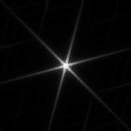
Bonus remark: A particularly nice example of PSF is glare, which comes from the Fraunhoffer diffraction of the camera/eye aperture. Below you can see what happens when a glare PSF is applied to an HDR image. The actual implementation convolutes the IPSF (the radial-symmetric of the glare PSF) with the source HDR image.
Glare applied to an Arion render

Typical glare PSF for a 6-blade iris