The Error function (erf)
Here is the 1D Gaussian function:
\[G(x,\sigma)=\frac{1}{\sigma\sqrt{2\pi}}e^{\frac{-x^2}{2\sigma^2}}\]Put in short, the Error function is the integral of the Gaussian function from \(0\) to a certain point \(x\):
\[\mathrm{erf}(x)=\frac{2}{\sqrt{\pi}}\int_{0}^{x}{e^{-t^2}}\mathrm{d}{t}\]At least, this is the way the formula is presented by Wikipedia and Wolfram Alpha for \(\sigma=1\). But as soon as you try to work with it you find out that in order to really match the above Gaussian function, normalization and axis scaling must be taken care of:
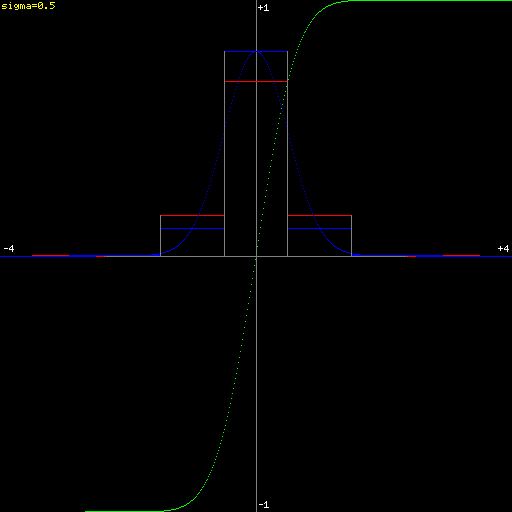
\[\mathrm{erf}(x,\sigma)=\int_{0}^{\frac{x}{\sigma\sqrt{2}}}{e^{-t^2}}\mathrm{d}{t}\]The plots below display \(G(x,\sigma)\) (bell-shaped) in blue, and \(\mathrm{erf}(x,\sigma)\) (S-shaped) in yellow.
A very typical use for \(G(x,\sigma)\) that I’ve been talking about on this blog lately, is to build convolution kernels for Gaussian blur. An image convolution kernel, for example, is a pixel-centered discretization of a certain underlying function (a Gaussian, in this case). Said discretization splits the \(x\) axis in uniform unit-length bins (a.k.a., taps, or intervals) centered at \(x=0\).
For each bin, this is pretty much the definition of the integral of \(G(x,\sigma)\) along the bin. That is, the increment of \(\mathrm{erf}(x,\sigma)\) between both end-points of the bin.
Discretized 1D Gaussian (\(\sigma=0.5\))
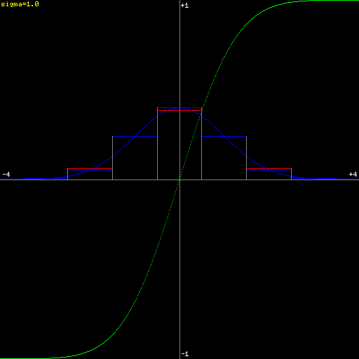
Discretized 1D Gaussian (\(\sigma=1\))
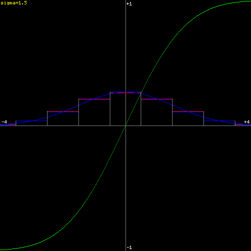
Discretized 1D Gaussian (\(\sigma=1.5\))
Doing it wrong
Most implementations of Gaussian convolution kernels simply evaluate \(G(x,\sigma)\) at the mid-point of each bin. This is a decent approximation that is also trivial to implement:
\[\mathrm{bin}(a,b,\sigma)=G(\frac{a+b}{2},\sigma)\]This value is represented in blue in the above plots.
Implementing erf
While \(G(x,\sigma)\) has a trivial explicit formulation, \(\mathrm{erf}\) is an archetypical non-elementary function.
Some development environments provide an \(\mathrm{erf}\) implementation. But most (the ones I use) don’t. There are some smart example implementations out there if you Google a bit. Usually they are either numerical approximations, or piece-wise interpolations.
Assuming that one has an \(\mathrm{erf}\) implementation at his disposal, the correct value for the bin \([a..b]\) is:
\[\mathrm{bin}'(a,b,\sigma)=\mathrm{erf}(b,\sigma)-\mathrm{erf}(a,\sigma)\]This value is represented in red in the above plots.
A poor-man’s approximation
If you are feeling lazy, an alternative approximation is to super-sample \(G(x,\sigma)\) along the bin. The amount of samples can be chosen to be proportional to how small \(\sigma\) is.
This method is easy to implement. However, it is far less elegant and also less efficient as more evaluation calls are required.
Conclusion
When discretizing a Gaussian function, as \(\sigma\) becomes small (close to, or smaller than \((b-a)\)), the approximation \(\mathrm{bin}(a,b)\) (in blue above) deviates significantly from the correct \(\mathrm{bin}'(a,b)\) (in red above).
So if you are going to Gaussian-blur at radius 1px or smaller, and precision is important, then it becomes necessary to use \(\mathrm{erf}(x,\sigma)\) or at least super-sample \(G(x,\sigma)\).