Downsampling and Gaussian blur
I talked about several strategies to optimize convolutions in some of my previous posts. I still got to talk about how to approximate a Gaussian blur using a multi-step Box blur in a future post. However, there is yet another good technique to optimize a Gaussian blur that may come handy in some cases.
This post is inspired by a need that I had some days ago: Say that you need to do a 3D Gaussian blur on a potentially humongous 3D data buffer. Working with downsampled data sounds ideal in terms of storage and performance. So that’s what I am going to talk about here:
What happens when downsampled data is used as input for a Gaussian blur?
The idea
Here’s the 0-centered and un-normalized 1D Gaussian function:
\[G(x,\sigma)=e^{\frac{-x^2}{2\sigma^2}}=e^{\frac{-1}{2}(\frac{x}{\sigma})^2}\]The sigma parameter in the Gaussian function stretches the bell shape along the x axis. So it is quite straightforward to understand that if one downsamples the input dataset by a scale factor k, then applies a (smaller) Gaussian where sigma’=s/k, and finally upscales the result by the same scale factor k, the result will approximate a true Gaussian on the original dataset where sigma=s.
In cleaner terms: if one has an input dataset (e.g., an image) I and wants to have it blurred by a Gaussian where sigma=s:
I'=Idownsampled by a certain scale factork.I"=I'blurred by a small Gaussian wheres’=s/k.J=I"upscaled by a scale factork.
How good is this approximation?
The Sampling Theorem states that sampling a signal at (at least) twice its smallest wavelength is enough. Which means that downsampling cuts frequencies above the Nyquist limit (half the sampling rate). In other words: Downsampling means less data to process, but at the expense of introducing an error.
Fortunately, a Gaussian blur is a form of low-pass frequency filter. This means that blurring is quite tolerant to alterations in the high part of the frequency spectrum.
Visual evaluation
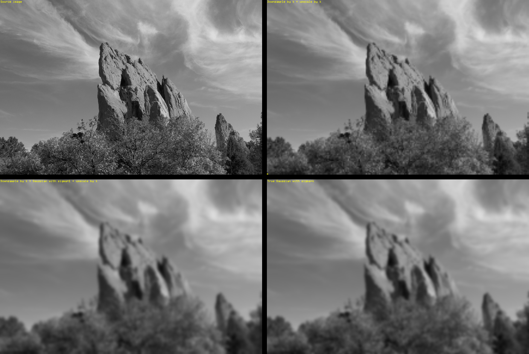
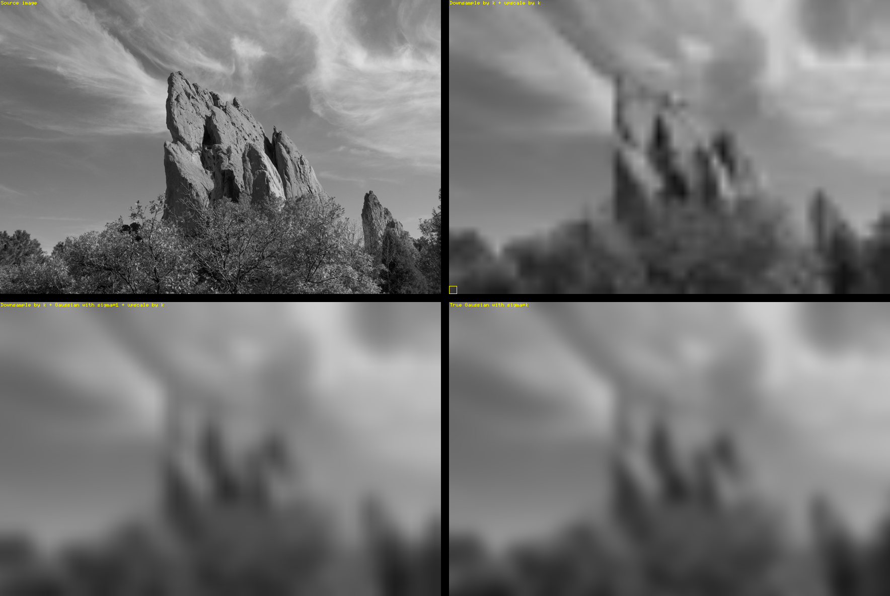
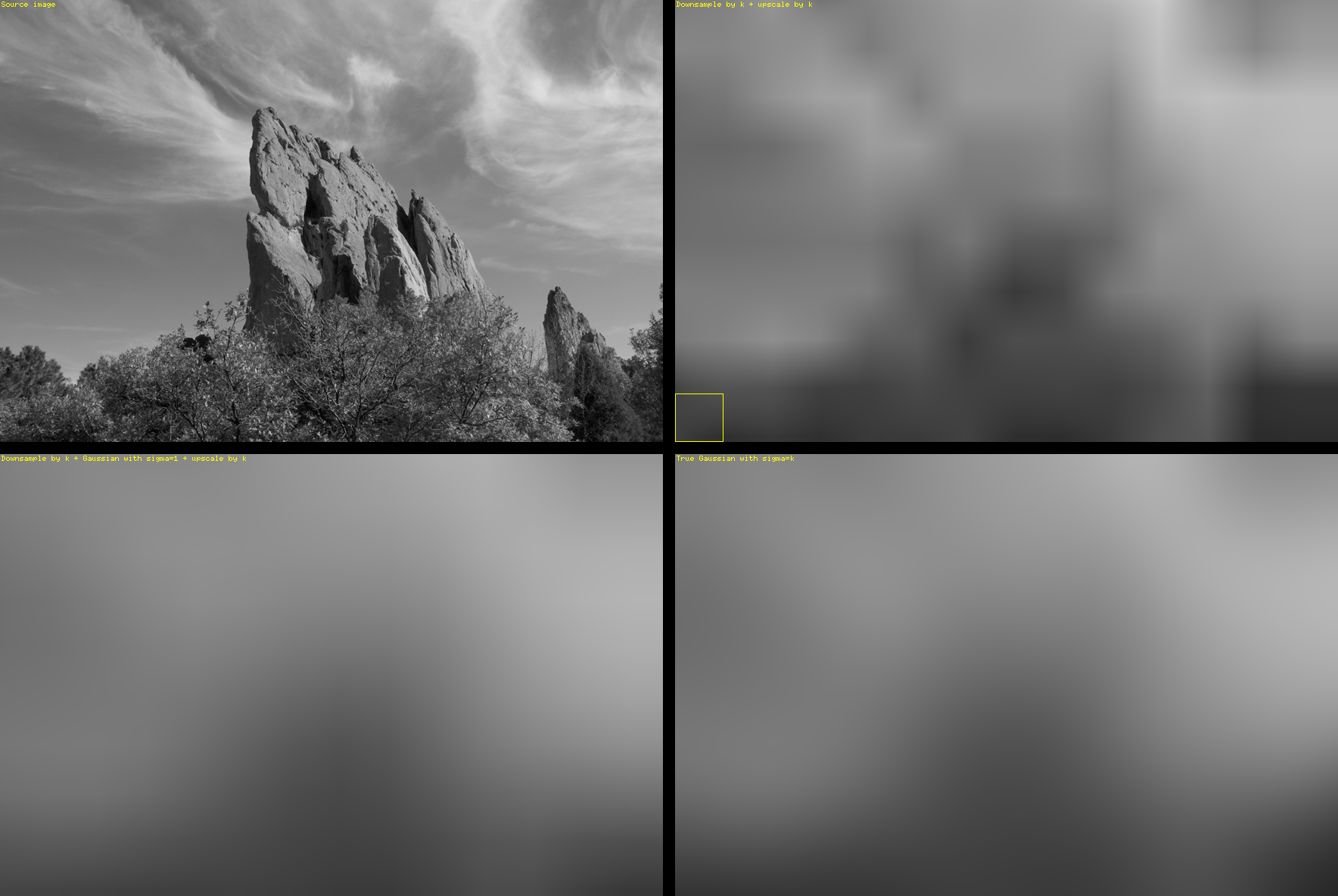
In the examples below I am downsampling with a simple pixel average, and I am upscaling with a simple bilinear filter. The 2x2 grids below compare:
- Top-left – The original image
I. - Top-right –
Idownsampled and upscaled byk(note the blocky bilinear filter look). - Bottom-left – The resulting image
J. - Bottom-right –
Iblurred by a true Gaussian wheresigma=s.
In these examples, k=sigma was chosen for simplicity. This means that the small Gaussian uses sigma’=1.
Gaussian blur where sigma=4
Gaussian blur where sigma=16
Gaussian blur where sigma=64
Conclusion
As shown, the approximation (bottom-left vs. bottom-right) is pretty good.
The gain in speed depends on multiple implementation factors. However, as I explained above, this post was inspired by a need to cope with a cubic memory storage problem when doing Gaussian blurs on a 3D buffer. Working with a heavily downsampled buffer clearly helps in that sense. And it is needless to say that decreasing the amount of data to process by k^3 also brings a dramatic speed boost, making it possible to use tiny separable convolutions along the 3 (downsampled) axes.
Note that one might pick any downsampling scale factor k>=1. The higher the value of k, the higher the approximation error and the smaller and faster the convolution.
The choice k=sigma offers a good trade-off between approximation error and speed gain as shown above.